This is a draft, do not read it unless you have been invited to

Content

• Beginning of tutorial
• Thermodynamic modeling of phase diagrams
• Some basic rules and terminology"
• Unary phase diagrams
• Property diagrams
• Binary phase diagrams
• Ternary phase diagrams
• Liquidus surface and other 3D diagrams
• Phase diagrams for special applications
• Multicomponent phase diagrams
• Literature
• Index

Phase diagram tutorial

This tutorial will teach you all you really want to know about phase diagrams and maybe a little more. If you are uncertain about your termodynamic knowledge please first follow the crack course on thermodynamics and modeling

Even if you are just interested in understanding binary phase diagrams you should follow carefully the sections on unary and modeling first. Unary diagrams are simpler than binaries and many facts and terms will understood more easily for unary systems and using thermodynamic models. In the binary section you are expected to be familiar with many terms first explained in the unary and model sections.

It is the hope of the author that when you have reached the binary section you will be so interested to read also the ternary and multicomponent section because these diagrams are the really useful ones and they are, in fact, much simpler than the binary phase diagrams.

The difference between 2-dimensional diagrams in general and phase diagrams

In almost all 2-dimensional scientific diagrams you have come across until now the lines in a diagram express some explicit functional relationship between the dependent variable (usually the x axis) and independent variable (usually the y axis) like y=f(x). This is not true for phase diagrams.

A phase diagram is more like a map. On a map you do not expect any relation between the x and y coordinates of the line defining the border between land and sea or between two countries for eaxmple. In the same way the lines in a phase diagram do not express any relationship between the two axis variables. The lines in a phase diagram simply separate regions with different sets of stable phases at equilibrium. The condition of equilibrium is the reason thermodynamics and phase diagrams are closely connected. Later, when you feel confident using equilibrium phase diagram, we will show you how to and understand phase diagram when the phases are not in full equilibrium ...

---

You may also have dealt with functions of several variables and found it difficult to visualize things in more than 3 dimensions. On the other hand, if you learned quantum mechanics you are familiar with reciprocal space with an infinite number of dimensions so then it should be no problem to handle realities than cannot be visualized in just 2 or 3 dimensions.

The thermodynamic properties of the phases vary with the state variables used as axis in the diagram and a new phase may become stable, or a stable phase may become unstable, at a certain set of values of these axis variables. Such a change of the set of stable phases is a point on a line in the phase diagram. As the properties of phases vary continuously the point will become a line, surface or hyper-surface when varying the one, two or more axis variables.

Most phase diagrams are 2-dimensional because that is the most easy to draw. But one may draw 1-dimensional and 3-dimensional phase diagrams although the latter kind is more for show. In reality the dimensionallity of a phase diagram for a system is determined by Gibbs phase rule (explaned later) which states that the dimensionality (in most cases) should be equal to n+1 where n is the number of components. So only unary systems can be drawn completely in a 2-dimensional phase diagram. But if pressure is kept constant can use 2-dimensional phase diagrams also for binary systems. Most real systems have many components and one has to section or project the real multidimensional phase diagram in different ways to obtain a 2-dimensional phase diagram

---

The 1-dimensional phase diagram for pure H2O at 1 bar is shown in this figure. At varying temperatures this molecule can be solid (ice), liquid (water) and gas (steam). The temperatures for these transformations is shown by tic marks on the temperature axis. This phase diagram is shown here as we have all experience of the phase transformations associated with water. Note that the transformations from ice to liquid water (freezing point) and from liquid to gas (boiling point) occurs at a specific temperature. We know there are many properties that vary with the temperature for example the volume. In the next diagram, which is not a phase diagram, the volume of water is shown as a function of temperature. Note that there are discontinuities in the volume at the temperatures where the phase changes. This is because the properties of each phase depend on its structure and the volume of H2O as ice, liquid and gas are independent of each other. The figure is drawn by hand and the changes are not to scale. You can notice the volume of ice is larger than that of liquid water at the freezing point which means that ice floats on liquid water. The volume change from liquid to gas is much larger and the gas has a larger volume at 100 oC than the same amount of liquid. If we allow the pressure to vary the temperatures for these transformations will change. At low pressure at high altitude the boling point is much lower as a phase with large molar volume becomes more stable at low pressure. The volume change associated with the freezing is much smaller and the freezing point is not affected so much. But as the volume of ice is higher than that of liquid the freezing point increases also with lower pressure. The temperature-pressure phase diagram of H2O will be discussed later. Adding another component to the system will also change these transformation temperatures. And that is the main topic in all 2-dimensional phase diagrams shown later.

The 1-dimensional phase diagram for H2O.

Volume as function of temperature for H2O. This is NOT a phase diagram.

The diagram to the right is the binary phase diagram for the Ag-Cu system at atmospheric pressure. For easier explanation the different areas have been colored, in most other cases all areas will be white. The vertical borders of the diagram are the pure elements. At low temperature both pure elements are solid and can dissolve a small amount of the other element, those areas are yellow. At some temperature the elements melt and in the upper red part the liquid phase is stable across the whole system. When crossing one of the lines from the yellow or red to the blue areas one has two phases stable, in this case liquid and either solid Ag or Cu. Finally in the green area, below the horizontal line connecting the two yellow areas and the lowest point of the red area, one has two solid phases. One of the solid phases is almost pure Ag and the other almost pure Cu. The mutual solubility decreases at lower temperature as the yellow areas becomes more narrow (and the green wider). The first important step in understanding 2-dimensional phase diagram is that it consists of different kind of areas with different number of stable phases.

In a single phase area there is a single phase stable for the values of the axis variables. For a point in an area with two or more phases stable there is no phase stable for the values of the axis variables for the point but one has a combination of two or more phases with properties that can be added together to give the axis value for the point. And in some important cases one can still deduce the properties of the stable phases.

To give a taste of what will learn we show you a colored phase diagram for a multicomponent steel to the right. This alloy has 8 elements Cr, C, Co, Si, Mn, W, V and the rest Fe. The nominal composition, in mass (weight) percent is given below. It is a so called high speed steel used for for high temperature cutting for example in drills and saws.

Each colored area has a different set of stable phases, there are up to 6 phases stable in some areas. The colors have been added to make the diagram it look nicer (or more lika a map). Areas with the same color does not have the same set of phases. The phase diagram is not exactly for this alloy as the carbon content is varying along the horisontal axis, but the diagram is useful because carbon is a very light element and can easily diffuse in or out of the material and as you can see the set of stable phases changes a lot with the carbon content. The vertical axis is the temperature in Kelvin and it is useful to know the phase changes when the material is heated and this kind of material may be used up to 1000 K without loosing its hardness. The content of the other alloying elements, except Fe, is constant in the whole diagram.

C Co Cr Mn Mo Si V W Fe 1.1 8 4 0.3 9.5 0.3 1.1 1.5 rest

These multicomponent phase diagrams can be calculated from databases with assessed thermodynamic models and that is why there is a section on models in this tutorial. We will look at it again at the end of the course to understand it better.

You may not believe it but it is much easier to understand these kinds of multi-component phase diagrams that binary phase diagrams. One reason for that is that they can be used just to know the set of stable phases for the aqes values. In binary and ternary phase diagrams one can extract more information, for example the composition of the phases in equilibrium.

Along the lines separating the colored areas in the phase diagram at least one phase must be just stable, i.e. have zero amount. The lines are thus often called a ``zero phase amount'' or ``zero phase fraction'' (ZPF) lines. Two ZPF lines may meet and at that point at least two phases must have zero amount. Depending on the type of diagram one can draw different conclusions how the lines should extrapolate from this point.

In phase diagrams some of the points where the ZPF lines meet have a special importance. These points are called invariant points because the number of phases with zero fraction at these points is equal to the degrees of freedom in the phase diagram. Depending on the axis in the diagram an invariant point is sometimes an invariant line.

A big difference beween maps and phase diagrams are that a map always have distances as axis. In a phase diagram one can have either extensive quantities, for example composition or volume, or intensive quantities (potentials) for example temperature, pressure or chemical potential. This means that the lines has to be interpreted sligtly differently depending on the the axis of the diagram.

Another big difference is that a 2-dimensional phase diagram, except for unary systems, is always a section or projection of a multi-dimensional reality. This means there are things "hidden" outside the plane of the diagram that it is sometimes useful to be aware of.

A summary of the lines in a phase diagram:

• A 2-dimensional phase diagram, like any map, consists of areas separated by lines. In all phase diagrams the "fundamental" lines are all ZPF lines (except the borders of the diagram). Note that a ZPF line may have more than one phase with zero fraction along the line, for example when the axis are potentials.

  But quite often those who draw phase diagrams like to put additional lines to explain other features like microstructures or metatstable states. It may take some experience to identify the ZPF lines from other added lines.

• In phase diagrams with the composition along at least one axis, some of the ZPF lines are known as solubility lines. A solubility line is the border of a single phase region giving the limit of solubility of a component in that phase. As the solubility line is also a ZPF line the amount of another phase is zero along the solubility line. But in general the ZPF lines are not solubility lines.

• You will often find another important kind of line in the phase diagram that is called tie-line. A tie-line connects two phases in equilibrium across a two-phase region. In some ternary phase diagrams one can even have "tie-triangles" which means that three tie-lines join the 3 phases in equilibrium as a triangle and inside the triangle one has 3 phases stable.

• It is possible for a tie-line to coincide with a ZPF line. An important case are the "invariant lines" in binary phase diagrams with temperature and composition as axis. The line representing the invariant equilibria at constant temperature joins together 3 phases in equilibrium. This invariant line can be split into 3 different ZPF lines and 3 different tie-lines, and this tutorial will make this fact very easy to understand.

In multicomponent systems one can have more than 3 phases in equilibrium and at the end of this tutorial you will be able to visualize multidimensional "tie-planes" joining together compositions of 4 or more phases in equilibrium. But do not worry, they will never appear as lines in phase diagrams.

• Unary phase diagrams
• Binary phase diagrams
• Potential phase diagrams
• Isothermal phase diagrams
• Ternary phase diagrams
• Liquidus surface diagrams
• Phase diagrams with tie-lines in the plane
• Multi-component phase diagram
• Isopleth phase diagrams
• Quasi-binary or quasi-ternary phase diagrams

Many of these types are overlapping but they will all be explained in this tutorial. You may also have heard about other types of phase diagrams because people like to invent names for each particular feature like "eutectic phase diagram".

Experimental determination of phase diagrams

Example coffee+sugar and water+salt

More advanced experimental techniques

Thermodynamic modeling of phase diagrams

We will frequently refer to thermodynamic models to describe the origin of different features of the phase diagram. It is much easier to explain them this way and the development and use of multicomponent phase diagrams is impossible without thermodynamic modeling. Please follow the crack course in thermodynamics if you feel uncertain about this subject.

For the modeling of phase diagrams the Gibbs energy per mole components G_m(T,P,x_i ) is the most frequently used thermodynamic function because most phase diagrams is at fixed pressure. Only in very special cases, like the phase diagram for pure water, Helmhotz energy per mole component A_m(T,V,x_i ) must be used because the Gibbs energy cannot handle a miscibility gap in volume.

• the gas and liquid are examples of phases without long range structure but with uniform composition in space. However, one can have several liquids, consider for example olive oil and vinegar, they do not mix even if you shake them forever the droplets of each liquid will just become smaller. This is an example of a liquid miscibility gap.
• In the solid state a phase must have a uniform structure and composition. There are many different crystalline structures possible for the atoms and each of these represent a different phase. So there is an infinite number of solid phases but, a relief, in a phase diagrams only a few of them will appear as stable (but if one is interested in metastable phase diagram one can have many more phases).

A phase must have a continuous Gibbs energy function and the first and second derivatives of the Gibbs energy, must also be continuous, there can be no discontinuety in any quantity for a single phase. If one has such a discontinuety that is an indication of a phase change. The Gibbs energy per mole, G_m of a phase is usually very smooth function of T P and composition. Also the derivatives of G_m, i.e. entropy, volume and chemical potentials, are often very smooth.

---

The second derivatives of the Gibbs energy, i.e. the heat capacity C_P thermal expansivity \alpha, isothermal compressibility \kappa and the stability function \omega must be continuouos but can have more drastic changes. The third derivatives of G_m for a phase does not have to be continuous.

An example of a drastic change in the heat capacity is shown in Fig.~\ref{fg:cpiron} for the heat capacity for pure iron. The ferromagnetic transition in bcc makes the heat capacity approach infinity at the Curie temperature. But according to theory the heat capacity must be continuous. Another example is the stability function shown in Fig.~\ref{fg:b2} which shows its value in the B2 phase in Al-Ni.

In all kinds phase diagram the total amount of the components is irrelevant, one has the same equilibrium if the system is 1 mole or 1 g. The system size is denoted N for moles and B for mass.

For systems with 2 or more components one can also vary the composition of the system (as noted earlier the total size is irrelevant for the equilibrium). The amount of different components is denoted N_i or B_i for the number of moles or mass of component i. Most often the amounts is not given as total number but as fraction or percent and the notation is x_i for mole fraction and w_i for mass fraction. There is no shorthand notation for mole or mass percent. For computer input and output italics and indices can usually not be used and the notation x(i) and w(i) is used.

The composition of a system may also be varied through $\mu_i$, the chemical potential or a_i, the activity, of component i. The chemical potential is defined as the partial derivative of the Gibbs energy relative to the amount of the component, keeping T, P and the amounts of all other components fixed.

Most phase diagrams are for constant pressure and for varying T and one composition, x_i of the system. But note that in physics phase diagrams are often calculated for constant V and varying activity a_i. This may lead to some surprising relations

The thermodynamic variables always appear in pairs, like T and S, P and V and N_i and $\mu_i$ in the expression for the Gibbs energy

where the latter is written for one mole of material. In each pair one variable is extensive and the other intensive.

Some basic rules and terminology"

The Gibbs phase rule applies strictly only to phase diagrams with only potentials as axis variables. If one has an extensive variable as one axis, like in most binary phase diagrams, one must apply the rule with some care.

In a two-phase region there are two phases stable. In the two-phase region one can always draw tie-line connecting the points representing the phases that are in equilibrium. Depending on the type of diagram one can be in the plane of the diagram and even parallel to one of the axis or it can be outside the plane. The word "region" means that for (small) changes of the axis variables one will still have the same set of stable phases but their amount and composition may change.

A tie-line is a line that ``ties together'' phases that are in equilibrium. The German name ``Konod'' is also often used. In binary phase diagrams with temperature and composition on the axis one can fill the two-phase regions with horisontal tie-lines connecting the phases that are in equilibrium.

A tie-line should be a straight between the phases in equilibrium but in some diagrams, that are not really phase diagramsm but may look like and be used as, the tie-lines can be curved.

Unary phase diagrams

We will first consider unary phase diagram, i.e. phase diagrams for a single component. The component can be a pure element like Cu or Fe or a very stable molecule like H2O. The Gibbs energy in a unary system depend only on T and P. The T-P diagram for pure Fe is given to the right. Fe has two cristalline forms at atmospheric pressure, bcc and fcc. At high pressure one can have Fe in a hcp lattice. In a unary phase diagram with T and P as axis the Gibbs phase rule can be applied without problems. The areas in the diagram represent single phase regions and there we have f=1-1+2=2 degrees of freedom meaning we can vary both T and P (within limits) and still have the same stable phase. Along the lines in the diagram we have 2 phase stable and f=1 meaning that there is a relation between T and P and only one of them can be varied to keep both phases stable. Finally at the points where the lines meet we have 3 phase stable and these points are invariants and can occur only for a fixed combination of T and P. As there are many different crystalline forms of Fe there are also several triple points, each occuring at its unique set of T and P.

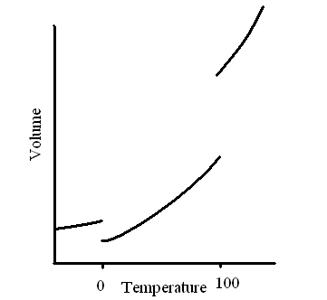
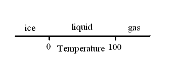
The lines in the T-P diagram are ZPF lines but there are two phases with zero amount along the lines! As T and P are intensive variables the change from one phase to another across a line is immediate but what is not shown in this diagram is that crossing a line means a change in volume and requires or releases an amount of heat. We know that it requires heat to melt ice and a mixture of ice and water remains at the same temperaure, 0 ^oC (at atmospheric pressure) until all ice has melted.

Question: Why are there always 3 lines meeting at each invariant point in the Fe-TP phase diagram?

• a) because there are 3 phases stable at the point and one of these phases is stable along each line.
• b) because there are 3 phases stable at the point and each line represent the exclusion of two of these.
• c) because there are 3 phases stable at the point and each line represent a combination of two of these.

With thermodynamic models for the different phases one can easily plot the diagram for Fe using the conjugate quantities, S and V. The T-V diagram in Fig.~\ref{fg:fetv}. In the Fig.~\ref{fg:fetv} one should note that the phases in equilibrium have different molar volumes and thus each single line in the Fig.~\ref{fg:fetp} diagram becomes two lines. The points representing the equilibrium between the two phases are connected with tie-lines. In this diagram all tie-lines are horisontal but in other diagrams the tie-lines across a two-phase region may have any direction or even be curved. In the diagram there are two separate two-phase regions fcc+bcc that suddenly end. The end points represent atmospheric pressure where the calculation has stopped. Even if one had calculated to zero pressure the two-phase regions whould not have extended much longer. But if one had calculated for negative pressures, i.e. assuming an isotropic force pulling the material, one could have made the two two-phase regions join together, provided the material would not have broken before.

Question: Why is there a gap between the two two-phase regions fcc+bcc?

Question: Why are the tie-lines horizontal?

The word eutectic is greek and means originally ``fluent'' (lättflytande) and has been used to indicate the equilibrium where the liquid is stable ?????

Question: What is the important physical effect of the density of ice lower than liquid water?

Question: Another less important effect?

A phase with a miscibility gap can exist simultaneously with (at least) two different sets of some extensive variables, for example volume or composition. One example is the H₂O system for which one can pass from the gas to the liquid state at high pressure and temperature. This means that above a certain limit of temperature and pressure gas and liquid is the same phase, usually called fluid.

Unless you work with fluids, either in geology or in steam generators, you will much more frequenly come across miscibility gaps where the phase can exist at the same time with (at least) two different compositions. Such miscibility gaps exists in the liquid and solid phases and they may often be metastable because other phases are more stable.

Question: Can one have a phase with a miscibility gap in S?

Describe the invented unary with S1, S2, liquid and gas

Property diagrams

Short about thermodynamic models, EOS for pure elements

There is a kind of diagram frequently used on its own or as complement to phase diagrams in thermodynamics that is called "property diagram".

Property diagrams for the different phases of Fe

G and V and S and Cp curves at constant P and varying T

G and V and S and Cp curves at constant T and varying P

Cp and Cv curves and their relation

Properties of the invented unary.

Show how a change of Cp for a phase affects the phase diagram (phase comming back at high T)

Show the risk of negative S or Cp when modeling

Question: Why is negative Cp impossible in a real phase?

CARNOT CYCLES

The steam engine and the refrigerator

Binary phase diagrams

The phase diagram you will find most often are the binary phase diagram with the composition on the x axis and temperature on the y axis and for constant pressure, usually at 1 bar. These diagrams are so common that some people think it is the only kind of phase diagram. But this tutorial have already shown you a lot of other kinds of phase diagrams and you will at the end of the tutorial you will find these diagrams almost trivial considering how many other kinds of interesting phase diagrams one can use.

The step from unary phase diagram to binary means one has one more component in the system. As already stated the size of the system has no influence on the equilibrium and normally one uses mole fractions, mass (weight) fractions or percent to give the composition. The composition is an extensive variable, the conjugate state variable is the chemical potential of the component. 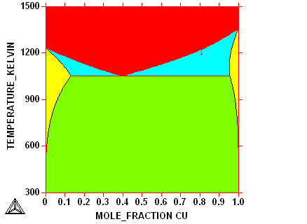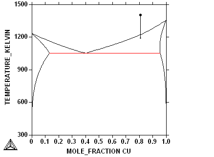Phase diagrams with a chemical potential axis instead of composition axis are very similar to a unary phase diagram, the regions are single phase and along the line there are two phases stable and where the lines meet there are invariant 3 phase equilibria, see Fig~\ref{fg:agcuat}. The same phase diagram plotted with a composition axis is shown in Fig.~\ref{fg:agcuxt}. Changing from chemical potential to composition is thus similar to change from pressure to volume in unary systems. We have horizontal tie-lines connecting the phases in equilibrium. c

But we are advancing a bit too fast, first let us go back and consider what it means to have two components mixing in the same phase.

In a gas phase the molecules can move freely and if the gas is ideal they are non-interactive and all collosions are elastic without loss of kinetic energy. In statistical mechanics one can derive the increase of entropy mixing two monoatomic gases of elements A and B and the following formula is found

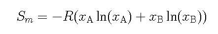
where x_i is the mole fraction of the element. Much time can be spent on explaining how different elements can be formed and one can formulate several chemical reactions between the elements but in the section on thermodynamics the Gibbs energy for an ideal gas with several molecules i is derived

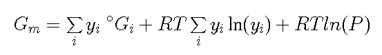
where y_i is the fraction of molecule i and ^oG_i is the Gibbs energy of formation of the molecule from the elements in their standard state.

---

From high school chemistry you may be familiar with writing chemical reactions between molecules and using equilibrium constants to determine their fractions but in computational thermodynamics with many components and molecules it is more convenient to describe the Gibbs energy of a phase with equations like this and the equilibrium is the same and the equilibrium constant can be calculated from the relevant ^oG_i.

Most of the phase diagrams we will deal with here will not include the gas phase, only liquid and solid phases. Non-ideal gases is not considered at all but can of course be modeled like the condenced phases although traditionally other types of models are used for fluids.

---

In the liquid phase that atoms are much closer than in the gas and there are attractive or repulsive forces between the atoms. If the atoms are interacting weakly one will have the same entropy of mixing as in the gas and the most used model for a metallic liquid phase is

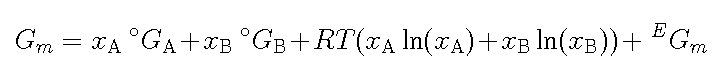
where ^EG_m describes the non-ideal part of the mixing. All these models and equations are described in more detail in the thermodynamics course

---

There can be many solid phases in a binary system and this will be discussed more later. All stable solid phases are crystalline i.e. the atoms are arranged in fixed lattices. Most of these are very simple like bcc, hcp and fcc shown in Fig.~\ref{fg:lattice1}. Only in special cases, like rapid quenching, can one obtain an amorpheous solid phase where the atoms are arranged randomly on space similarly to the liquid but contrary to the liquid the atoms cannot move around.

---

Even in crystalline solids the atoms can arrange themselves randomly on the available sites and simple statistics shows that one will have an entropy of mixing identical to that for an ideal gas. The Gibbs energy expression for a crystalline solid phase with substitutional mixing on the lattice is

This is identical to the model for the liquid! So there is no real difference between a substitutional model for crystalline phases and for the metallic liquid phase. We will later find cases when the lattice have several different types of sites and where the atoms does not mix randomly but for many simple cases the equations above are sufficient for modeling the thermodynamic properties of a phase.

There are a few binary systems with complete solubility in liquid and solid. One case is shown in this figure. One requirement for this to happen is that the two pure element have the same crystall structure as solid, both Ge and Si have the diamond structure with Strukturbericht A4. But that is not enough as will be shown later. The curves joining the melting points for the two pure elements are called solubility curves and between the curves one have a two-phase region where liquid and solid phases coexist. In this two-phase region one has tie-lines joining the phases that are in equilibrium at a given temperature. The composition of the phases at the end of the tie-lines are given by the points on the solubility curve. At different points on the tie-line one have different amounts of the two phases.

An alloy with a given composition will thus on heating start melting at its liquidus temperature and on cooling from a liquid state it will start solidifying at the liquidus temperature.

At the melting point for Ge in Fig.~\ref{fg:sige} a small addition of of Si will increase the melting point. For the pure elements the transformation from liquid to solid occurs at a singe temperature but for an alloy with both elements there will be a solidification interval where the liquid and solid will coexist over a temperature range, called the solidification interval, see Fig.~\ref{fg:gesi2}. At the Si side the solubility curves join each other at the melting point for pure Si.

In some applications, for example soldering, one is interested in as small solidification interval as possible. In casting of metals it is often convenient to have as small solidification interval as possible to avoid shrinkage and pores in the cast. See also the section on segregation later.

It is not obvious that an addition of an element with a higher melting temparure will increase the melting temperature. In Fig.~\ref{fg:crfe} for the Cr-Fe system show that one may have more complicated behaviour with a minimum (or maximum in other cases) in the liquidus curves.

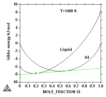
The Gibbs energy curves for the liquid and the diamond (A4) phase at different temperatures are shown in the figures below.

At a high temperture, 1800 K, the system is liquid across the whole system. and that is evident because the Gibbs energy curve for the liquid phase is lower than that of the A4 (diamond) phase at all compositions. From the diagram one can also obtain the chemical potentials of the components by taking a tangent to the lowest Gibbs energy curve at any composition and read the values of the Gibbs energy for the pure elements at the end points of the tangent.
At an intermediate temperature, 1400 K, the Gibbs energy curve for the liquid is lower at the Ge side and increasing the Si content the curve will cross that for the diamond (A4) phase and at the Si side the diamond phase will be stable. The most stable state is that with the lowest Gibbs energy and in figure the common tangent between Gibbs energy curves for liquid and A4 is drawn (green line). For the composition range between the points of tangency, marked with triangles in the figure, system has its lowest Gibbs energy by separating into two phases, liquid and A4. For compositions to the left of the left tangency point the system is liquid, for compositions to the right of the right tangency point it is solid (A4). Between the points of tangency the composition of the phases are constant and the amount of the phases changes with the composition axis. If you click on the diagram you will get the lowest Gibbs energy at any composition marked as a read curve in the single phase regions and as green in the two-phase regions. The chemical potentials of the components inside the two-phase region are constant as the the tangent is constant. This is true for binary systems, for higher order systems it is not true.
At the lowest temperature the system is solid at all compositions and the Gibbs energy curve for the A4 phase is lower than that for the liquid at all compositions.

All ZPF lines in all phase diagrams represent such common tangent constructions. In ternary and higher order systems there will be tangent planes or hyper-planes, where the Gibbs energy curves of the co-existing phases have a plane in common. This is a consequence of the fact that the chemical potentials of all elements must be the same in the phases that are in equilibrium. When modelling phase diagram this can be used as information to determine the model parameters of each phase.

The point of crossing between the Gibbs energy curves is not without importance. When an alloy is rapidly quenched equilibrium cannot be established and the crossing point marks the composition for which the alloy can be transformed from liquid to solid (A4) without any diffusion. For solid state transformations such "T-zero" or T₀ points can be important to control diffusionless transformation like martensite in steels.

We will now look at the connection between the phase diagram and the microstructure for a simple eutectic phase diagram. We will assume that the solid phases will form dendrites and there will then be a cooperative eutectic growth. In the figures below you will be able to see simultaneously how the composition of the phases in the phase diagram and the microstucture changes during the cooling. In the 3rd frame you can select yourself a quantity to plot.

First select composition

phase diagram	microstructure
	user selected: DTA curve
third question	answer

Eutectic phase diagrams. Microstructure at various compositions

Peritectic phase diagrams. Microstructure at various compositions

T-x and T-mu diagram

show G-x diagrams for variable T and corresponding T-x (movie?)

allow student to enter model paranmeters and calculate G-x and T-x diagrams

Other special invariants (monotectic, congruent melting ....??)

Liquid miscibility gap

Solid miscibility gap, metastable miscibility gaps

Modeling binary phases. Lattice stabilities, heat capacity of intermetallic phases (Kopp-Neuman). Gibbs energy of mixing. Examples of calculated diagrams with different parameters.

Phases with restricted solubility

Intermetallic phases

Phase diagrams with several features

Chemical ordering

Solid state transformations, eutectoid, peritectoid etc

Carbides, oxides etc

Metastable phase diagrams

Scheil-Gulliver solidification simulation

Variable pressure

Quasi-binary phase diagrams

Ternary phase diagrams

Isothermal section

Projections and sections

Ternary Isopleth diagrams (Al-Mg2Si)

Solubilities of third element in binary phases

Ternary phases

Ternary diagrams with fix activity

Liquidus surface

3D phase diagrams

Gibbs energy surfaces

Phase diagrams for special applications

Para-equilibrium phase diagrams

Phase diagrams for geological systems including high pressure

Multicomponent phase diagrams

Isopleths

Property diagrams

Congratulations! You have finished the tutorial and your score is very good ???? . You have the now the necessary background to use phase diagrams in your future studies or other work.

Literature

Index

Not in any particular order

• General diagrams and phase diagrams
• Zero phase fraction lines
• Crossing zero phase fraction lines
• Types of phase diagrams
• Modeling phase diagrams
• What is a phase
• Why must the thermodynamic properties of a phase be continuous?
• System size
• State variables
• Composition variables
• Conditions
• Gibbs phase rule
• Single phase region
• Two phase region
• Tie-line
• Unary phase diagram
• Unary phase diagram with T and P axis
• Unary phase diagram with T and V axis
• Unary phase diagram with S and P axis
• Unary phase diagram with S and V axis
• Temperature dependence
• Pressure dependence
• Fluid
• Eutectic equilibrium
• Congruent point
• Consolute point
• Phase diagram for water and steam
• Miscibility gap
• Property diagrams