1 Introduction

This is an dynamic summary to keep everyone involved updated with the current development of the 3rd generation of the Calphad unary database. It also contains unresolved issues and ongoing discussions in Appendices.

The aim is to make the new thermodynamic databases closer to the physical reality while keeping them useful for demanding engineering applications which need rapid calculation of equilibria and various thermodynamic properties in multicomponent systems. The current unary database using the 1991 SGTE unary database by Dinsdale [7] will continue to be used in parallel for the foreseeable future.

Section 2 is a very short summary of decisions and unresolved issues, usually with a short motivation. We should keep this short and use the Appendices for detailed explanations, expressing different opinions and discussions.

At present the Appendices are mainly my personal view of things, but everyone should express their opinions there. All mistakes should also be recorded, otherwise we will make the same mistakes over and over again.

2 Executive summary of sub projects

The sub projects are closely related, not independent.

1. Heat capacity zero at T = 0, for details see Appendix B.

   This is a mandatory physical reality for all phases.

   1. The Einstein model, is used to describe the low T heat capacity of all phases, stable or metastable. The Einstein model is preferred because it can easily be integrated to a Gibbs energy and even using a Debye model an additional polynomial in T is needed to fit experimental data.
   2. The additional polynomial in T must not have any terms in T with powers < 1 or T ln(T) and should not have any breakpoints.
   3. The Einstein model has a parameter, denoted θ, which is related to the phonon frequencies of the element. To fit the heat capacity of a pure element, a stoichiometric phase or an endmember of a solution phase, a sum of several Einstein functions with different θ and weight factors can be used. Normally the weight factors should sum up to unity (or the number of atoms involved).
   4. In a solution phase θ, or rather ln(θ), varies with the composition. For simplicity an element modeled with multiple θ should have a single θ selected to vary with composition, see Appendix B.1.
2. Entropy zero at T = 0, for details see Appendix C.

   The entropy of perfect ordered crystalline phases at T = 0 K must be zero according to the third law. Such a phase must not have any terms depending on T with power ≤  1 in its Gibbs energy expression.

   1. Crystalline phases that are not perfectly ordered at T = 0 K (for example an ideal solution or magnetite, Fe₃O₄, an inverse spinel) and the amorphous phase can have a positive entropy at T = 0 K, The opinion of Göran Grimvall can be found in Appendix C.
   2. Gibbs energy parameters for ordered endmembers and other Gibbs energies with linear T dependent coefficients can have these converted to an excess parameter for the θ parameter according to Dinsdale et al. [14], to reproduce the properties of the phase above θ. See Appendix C.1.
3. Model for magnetism, for details see Appendix D.

   The models by Qing [9] and Xiong [10] are accepted with minor modifications. This means separate Curie and Neel T but the proposal to have individual Bohr magneton number has been put on ice. Add some references of recent assessments!

4. Extrapolation of the heat capacity of liquids below their solidification T, for details see Appendix E.

   The liquid two-state model proposed by Ågren [5] and more recently in Becker et al. [11] is used. A recent assessment of Al-C is by Zhangting et al. [16].

   This model describe the amorphous and liquid phases with a single Gibbs energy function separated in two terms, G_M^amf and G _M^d.

   1. The low T amorphous phase, G_M^amf, is described by an Einstein model and a polynomial as explained in section 1 which may include a linear T term because it is not crystalline. G_M^amf is composition dependent and there can also be a magnetic addition [9].
   2. The transition from the amorphous state to stable liquid as well as the stable liquid itself is described by a composition dependent G_M^d parameter as a polynomial in T. This polynomial may include terms with T and T ln(T) because these have no contribution at low T.
5. Extrapolation of the heat capacity of crystalline phases above their melting T, for details see Appendix F

   The Equi-Entropy Criterion (EEC) proposed by Sundman et al. [15] is used to prevent the reappearance of crystalline solids extrapolated to high T. EEC replaces the breakpoint used in the SGTE 1991 unary database at the melting T of the solid phase of the pure elements by a software test of the entropy of solid and liquid phases. It has been used in the assessment by Zhangting et al. [16]

3 Some related topics

The fact that physical models has to be converted to moles per formula unit is explained in Appendix A. Modeling of thermal vacancies is discussed in Appendix G and molar volumes in Appendix H.

References

A The Gibbs energy per mole atom or formula unit

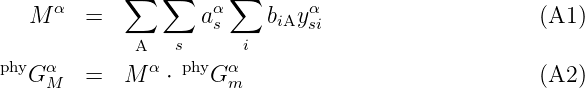
A model for the physical contribution to the Gibbs energy,  ^phyG _m, is normally per mole atoms indicated by the subscript m. However, the Gibbs energy models based on the compound energy formalism (CEF) [4], require the contribution per mole formula units of the phase. CEF use formula units because many phases contain vacancies or more complex constituents than the pure elements. In such a case the physical model function must be multiplied with the number of atoms/formula unit of the phase α,M^α, calculated as:

This fact has been ignored in earlier applications of the magnetic model resulting in nonphysical values of the Bohr magneton number for some phases, for example in the assessment of magnetite by Sundman [8].

B The Einstein model at low T

Integrating the Einstein heat capacity model

The Einstein model is preferred because it is simpler than any other model to integrate to a Gibbs energy. Even with a Debye model an additional polynomial in T is needed to describe the experimental data for each pure element.

The polynomial in T added to the Einstein function must not include terms with powers in T ≤ 1 or T ln(T).

It has been decided to use ln(θ) as composition dependent parameter. θ may possibly depend on P but must not depend on T.

B.1 Modeling with multiple θ parameters

In some cases a pure element, stoichiometric compound or endmember has its heat capacity fitted using multiple θ, for example pure C as graphite. A software provided function, GEIN(θ), with a single constant parameter, θ, can be used in the Gibbs energy expression for the endmember to calculate eq. B2 and its derivatives with respect to T for the endmember.

1. Bosses opinion:
   To avoid complications in solutions a single θ should be selected for each element or endmember to model the composition dependence even if the element itself is described using several θ. The reason is that:

   i) θ is an approximation of the phonon spectra,
   ii) the heat capacity data for solutions are not well known and
   iii) to avoid very complex modeling issues replacing linear T dependence in other Gibbs energy parameters by θ parameters.

   To do anything better than a single θ in solutions we should model the phonon spectra which is far outside the Calphad level of ambitions.

   A single θ, normally representing the major phonon frequency, can be selected as the composition dependent θ used in the explicit Einstein contribution. This contribution must subsequently be subtracted from the Gibbs energy functions fitted with multiple θ for the endmember.

C The entropy at T = 0 K

Evidently the 3rd law creates strong emotional argument. Some opinions below.

1. Göran Grimvall sent a few emails about the entropy at 0 K in August 2019. These are summarized and translated below.
   1. Pure elements and stoichiometric compounds without defects and which are dynamically stable have S = 0 when T = 0.
   2. Amorphous structures have finite entropy at T = 0 K, see below.
   3. Stoichiometric compounds with perfect structure but atomic disorder have finite entropy at T = 0 K (one can argue in the same way as for amorphous phases).
   4. Phases that are dynamically unstable at certain T and/or composition have neither a defined entropy nor Gibbs energy. In Calphad one can assign them any value as long as it does not have any consequences for the stable system. But it is reasonable to treat them similarly to metastable phases using S = 0 at T = 0 K and have positive Einstein T.

   For the amorphous phase:

   Consider a big piece of an amorphous system. Cut a large but finite part of this with N atoms. Call this piece A and consider it as a perfectly ordered unit cell. If A is repeated periodically we have a system with entropy 0 at T = 0 K. But we can also cut other parts in the big system, B, C, D etc all with N atoms. If any of these is repeated periodically we have a system with entropy 0 at T = 0 K. But this is not the case for an amorphous system. Instead it should be treated as a disordered system with parts A, B, C etc. This disorder means a finite entropy at T = 0 K. The larger the value of N the greater number of alternative parts B, C etc.

   Another way to argue: the entropy S = k_B ln(Ω) is a measure of the degree of disorder, Ω, i.e. the number of separate subsystems A, B, C etc. with practically the same energy. If N is large then Ω is also large but the number of subsystems, A, B, C etc. with N atoms in a given part of a large amorphous sample varies with 1/N. Thus there is a given entropy per atom in an amorphous sample.

2. Bosses opinion: If the entropy zero at 0 K for all phases was important for Calphad there would be no question about implementing it. But as Calphad has existed more than 50 years without even requiring that C_P = 0 at 0 K, it is not important. We now introduce C_P = 0 for all phases and S = 0 for perfectly ordered crystalline phases.

   Requiring that all phases, stable or metastable, must have S = 0 at T = 0 would mean Calphad cannot use its fundametal model, an ideal solution, because this will have S = ∑ _ix_i ln(x_i) at T = 0. We can wait another 50 years until the 4th unary to introduce S = 0 for any other kind of phase if we find it possible and necessary.

C.1 Converting linear T terms to Einstein θ

Following a proposal from Dinsdale et al. [7] to avoid non-zero entropy at 0 K means that any linear T terms in the classical Kaufman lattice stabilities [3] (and several later papers) can be converted to a Δθ for the metastable phase to avoid non-zero entropy for the metastable phases of the pure elements.

Linear T terms in endmembers, excess parameters and other parameters contributing to the Gibbs energy can also be converted to a parameter in the composition dependence in θ. In principle a coefficient for a linear T term “b” can be replaced by “b/3R” in a θ parameter with the same composition dependence to reproduce the properties of the phase above θ.

Some care should be used to avoid negative θ.

D The magnetic model

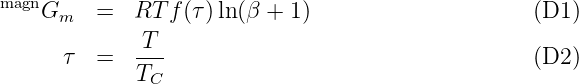
The contribution to the Gibbs energy due to the magnetic properties per mole atom is:

NOTE the current functions f(τ) etc. should be added.

The magnetic eq. D1 should be multiplied by M^α, see Appendix A, when used per mole formula unit.

There are separate Neel and Curie T and it is quite surprising to find that for a magnetic element the Neel and Curie T should have identical values but with opposite sign!

Individual Bohr magneton numbers for the elements is not adopted yet. The same Bohr magneton number is used for ferro- and antiferromagnetism as well as any kind of magnetic contribution.

...unfinished, some recent assessment references needed

E The liquid two-state model

The liquid phase is described using a two-state model described in Becker et al. [11].

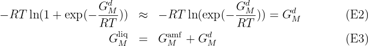
This model has a Gibbs energy description including an Einstein heat capacity contribution for the metastable low T part of the liquid, G_M^amf, assumed to be an amorphous phase. It has also a parameter, G_M^d, describing both the transition to the liquid phase and the stable liquid above the melting T of the element:

In the amorphous state at low T the term exp(-) should approach zero (i.e. G_M^d should approach very large positive values) and the second term in eq.E1 can be ignored. For the stable liquid exp(-) should be much larger than unity (i.e. G_M^d should approach large negative values) and second term becomes:

In the G_M^amf parameter one can use a linear T term because the amorphous phase may have nonzero entropy at 0 K. But no T ln(T) and no T powers less than 1 because the amorphous phase must have zero heat capacity at T = 0 K.

The G_M^d parameter should change from positive to negative values in the amorphous state and this can generate a heat capacity contribution. In the G_M^d parameter both linear T and T ln(T) terms are possible because they will not give any contributions at T = 0 K.

The parameters for the liquid two-state model, G_M^d, can be very different for elements with different melting T, for example Al and W [13]. Great care should be taken determining the G_M^d,

Composition dependent parameters for the stable liquid can be used in both G_M^d and G_M^amf but usually very little is known about the amorphous phase. Interaction parameters in the G_M^d can have linear a T term as it will not influence the low T properties.

F The equi-entropy criterion, EEC

The breakpoint at the melting T for the pure elements in the 1991 SGTE unary was an emergency fix to avoid that solid phases, which normally have an increasing heat capacity before melting, would become stable again when this increase is extrapolated to higher T. This will happen if the extrapolated heat capacity of the solid is larger than that of the liquid, which normally is fairly constant around 3R at high T. In the 1991 SGTE unary the heat capacity of the extrapolated solid was forced to approach that of the liquid above the breakpoint. The breakpoint represents a kind of 2nd order transition in the solid and it solved the primary problem but created others, for example strange heat capacity curves for compounds with their heat capacity modeled with the Neumann-Kopp rule [1, 2] and with higher melting T than a constituent element.

The similar breakpoint for the liquid, to avoid that the liquid becomes stable at low T, is removed by the liquid two-state model, see Appendix E. But there is no similar way to prevent the heat capacity of extrapolated solid to increase.

Instead a well established experience that the liquid is always the condensed phase with the highest entropy in a system, is used. This is a natural consequence of the fact that the liquid will become more stable than any solid phase at increasing T. An important observation is that this is independent of the phase compositions.

The Equi-Entropy Criterion (EEC) proposed by Sundman et al. [15] is based on this observation. During an equilibrium calculation EEC will compare, at the same T, the entropy of the solid phases with the entropy of the liquid at their current compositions. If a solid phase is found to have higher entropy than the liquid the conclusion is that this solid suffers from a bad extrapolation of its heat capacity and the solid Gibbs energy must also be wrong and the phase is not allowed to be stable.

EEC does not require any modification of the Gibbs energy expression of the extrapolation of the solid phase but must be implemented in the thermodynamic software using the data. No breakpoint is needed in the Gibbs energy function of the solid but some care should still be used to avoid that the heat capacity increases very rapidly above its melting T.

It is not forbidden to introduce a breakpoint in order to use the data in a software where EEC is not implemented but such a breakpoint should be at an even 100 K above the melting T, to indicate it is a fictitious breakpoint, and the derivative of the heat capacity should be continuous at the breakpoint to avoid the resemblance with a 2nd order transition.

During the discussions of EEC there were attempts to define a “crystalline breakdown T”, which should be a few 100 K above the melting T but it was found difficult to handle for solution phases and abandoned. EEC is related to the “entropy catastrophe” criteria [6] for a pure compound but it is applied to cases when the solid and liquid does not have the same composition. It is simply based on the experience that no solid phase can be stable with a higher entropy than that of the liquid at the same T.

G Thermal vacancies

All phases has defects of different kinds and the thermal vacancies are important for simulating kinetic properties. The Gibbs energy for thermal vacancies in a phase, G_{V a}, should be:

There are several other proposals for thermal vacancies but it should be recognized that this energy is not related to vaporization or equilibrium with any other phase, most vacancies are created when atoms move to a grain boundary, dislocations or other crystalline defects.

H Modeling the molar volume

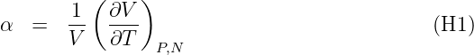
The volume is not included in the 1991 unary database but is of great importance. Some ideas:

1. The most recent discussion made me think that the thermal expansion of elements should be zero at T = 0? Maybe use an Einstein function for α?
   
   possibly with the same θ as for the heat capacity? The volume change is certainly associated with the vibrations, i.e. the Einstein θ.
2. Can we handle of the invar effect? Combine volume with magnetic model?